TMLE stands for Targeted Minimum Loss-based Estimator. It is a statistical estimator widely used in a pharmaceutical context, namemly to infer causal interaction between patients, a treatment and the outcome.
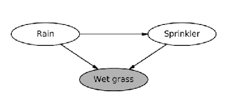
It makes use of what we call a "Structural Causal Model" (SCM). It is a (directed acyclic) graph that desribes the relation between random variables. From an example of Judea Pearl's book 1, if it had rained, the grass will be wet. The SCM says that the rains is a probable cause for the grass to be wet, alongside other causes, as shown in the image below.

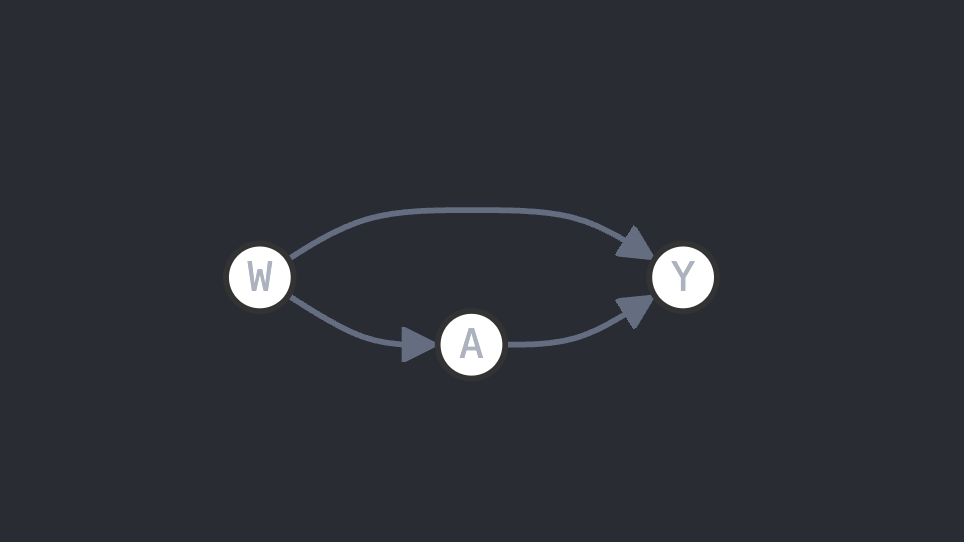
TMLE's SCM is simple: the model comprises three variables $\mathcal{O}=(W, A, Y)$ where $W$ is the covariate, i.e. the information about the patient, A is the treatment (0 or 1, the latter being "treated") and Y is the outcome (either a classification like death/alive or a predition like 12mg/L of white cells). In some litterature, W is written X and A is written W, sometimes another thing. Here, we follow the notations from Prof. van der Laan 2. We then assume the following interaction between the variables:

And that is why we need TMLE. One could say that we just need to fit a general model on A+W to predict for Y, but doing doesn't account for bias in assigning the treatment. If the intervention of a drug works better for, let's say, women than men, and that your study comprises more women than men, then your results would be very good, despite clear bias. Therefore, you need to account for such biases, and TMLE does just that.
It is very important to understand how A acts on the model. In a world with perfect data, we really want to measure the outcomes for both $A=1$ and $A=0$ for all of the covariates, to then draw perfect conclusions on the effect of the intervention. Unfortunately, we're on planet earth, and if I give a drug to someone I cannot undo that. And as we are trying to estimate the effect of A acts on the model, through what we call the Average Treatment Effect (ATE), we need to have the most sense of how our model interacts. The ATE then answer the following question: what difference could I expect in my outcome between people receiving the drug and people not receiving it. In maths, it yields: $$ATE=\mathbb{E}\{Y(1)-Y(0)\} = \mathbb{E}_{W}\{\mathbb{E}\{Y\mid A=1, W\} - \mathbb{E}\{Y\mid A=0, W\} \} $$ where $\mathbb{E}\{Y\mid A=1, W\}$ is the quantification of "what happens if people take the drug", $\mathbb{E}\{Y\mid A=0, W\}$ the quantification of "what happens if people do not take the drug", and taking the expetancy over their difference yields the expectancy over all of the covariates.
Throughout this tuto, some simple python code is given. We assume the following:
import numpy as np
# Define the numpy arrays and matrix
n = ...  # number of covariates
d = ...  # number of parameters
W = ...  # n x d matrix representing covariates
A = ...  # 1 x n array representing treatment assignment
Y = ...  # 1 x n array representing outcomes

# Define the GLM/LogisticRegression class with fit and predict methods
# in practice one should use sklearn.linear_models.LogistiRegression/AnyGLMRegressor
class GLM/LogisticRegression:

    coef_ = ... # list of the coefficints of the regression

    def fit(self, X, y):
        # Method to fit, takes X and y as arguments
        ...

    def predict(self, new_X):
        # Method to predict using a previous fit, takes new_X as argument
        ...

    def predict_proba(self, X):
        # Method to return the probability associated with the prediction for every covariates.
        # Only for LogisticRegression
        ...
# Instantiate the GLM class
glm = GLM()
ipw = LogisticRegression()
First, we need to fit some general model on the data, that is we need our "dummy" estimator to grasp a general sense of what's happening. Although this is very biased (like explained before), it still captures the general interaction between A and W, and will be useful for our debiasing process.
We do so by fitting a general linear model 3 on the design matrix $X=\text{hstack}(W,A)$ for outcome $Y$. In G-computation, we would then make our intervention here by predicting what would happen to each covariate now if we were to set $A=1$ or $A=0$ for each patient, to measure the ATE directly: $X_0=\text{hstack}(W,A=0)$ and $X_1=\text{hstack}(W,A=1)$, each respectively predicting $Y_{0/1}$, and $$ATE=\text{mean}\{Y_1-Y_0\}$$
As usual, here is a corresponding python code:
glm.fit(np.column_stack([W, A]), y)
Y_pred = glm.predict(np.column_stack([W, A]))
Y_1 = glm.predict(np.column_stack([W, np.ones_like(A)]))
Y_0 = glm.predict(np.column_stack([W, np.zeros_like(A)]))
ATE_G_comp = np.mean(Y_1 - Y_0)
Now that we have our fitted model, we can begin reducing the bias. The first step is to estimate what we call the propensity score model, which predicts the probability of receiving treatment given the covariates. This model is used to compute the Inverse Probability Weighting (IPW), which is widely used in causal inference. If we take again the example from the beginning, the propensity score model might predict that women have a 70% probability of being assigned the treatment. IPW takes the inverse of these probabilities and multiplies them with the observed outcomes. In our example, this would give more importance to men's results, who have a lower probability of treatment assignment. As a result, their "bad outcomes" will be more influential in the final analysis, leading to a less biased estimate.
To estimate the propensity scores, we fit a logistic regression to predict $A$ given $W$. This gives us $\mathbb{P}(A=1\mid W)$, the probability of being assigned treatment conditional on covariates. From these propensity scores, we can construct what's called the clever covariate H, which is a function that helps target our parameter of interest. The clever covariate takes the form $H = \frac{A}{\mathbb{P}(A=1\mid W)} - \frac{1-A}{1-\mathbb{P}(A=1\mid W)}$.
For TMLE, we use both the propensity scores and clever covariate in the targeting step (section 3). Here is the python code to compute these quantities:
ipw.fit(W, A) # Fit propensity score model
g1W = ipw.predict_proba(W)[:, 1]
H1W = 1/g1W
H0W = -1/(1-g1W)
H = A/g1W - (1-A)/(1-g1W) # The clever covariate
The targeting part is central to TMLE. What we call the targeting is an estimate of how much ($\hat{\epsilon}$) we need to update our initial outcome model predictions ($\hat{Y}$) with respect to the clever covariate ($H$) to reduce bias. Mathematically, we solve:
$$\hat{\epsilon} = \argmin_\epsilon\ \mathbb{E}[Y \log(\text{expit}(\text{logit}(\hat{Y})+\epsilon H)) + (1-Y)\log(1-\text{expit}(\text{logit}(\hat{Y})+\epsilon H))]$$
This corresponds to fitting a single-parameter logistic regression of $Y$ on $H$ (without intercept), where $\text{logit}(\hat{Y})$ acts as an offset. The $\text{expit}(\text{logit}(\hat{Y}) + \epsilon H)$ corresponds to a first shift from the predicted outcome $\hat{Y}$ into a probability space through the logit, then offsetting it by $\epsilon H$, which is the debiasing, and then shifting back to the prediction space with expit. We then take the correlation between $Y$ and $1-Y$ and those rearranged approximation and we take the minimum over such $\epsilon$.
Once the targetting estimator is fitted, we can update our expected outcomes accordingly, by offsetting the predicted outcomes $\hat{Y}_{0/1}$ with $\hat{\epsilon}H$ to get $Y^*_{0/1}$. As usual, here is the corresponding python code:
eps = LogisticRegression(fit_intercept=False).fit(H.reshape(-1, 1), Y).coef_[0]
Y_1_star = Y_1 + H1W*eps
Y_0_star = Y_0 + H0W*eps
Finally, we can compute the ATE! We just compute the mean difference between $Y_1^*$ and $Y_0^*$.
ATE = np.mean(Y_1_star - Y_0_star)
Judea Pearl. 2000. Causality. New York: Cambridge University Press. ↩
Mark J. van der Laan and Sherri Rose. 2018. Targeted Learning in Data Science: Causal Inference for Complex Longitudinal Studies (1st. ed.). Springer Publishing Company, Incorporated. ↩
using a GLM to fit our model ensures statistical properties are indeed respected, like the need for our model to support a normal distribution. []: One could fit other ML models, but that would require more care in the model's assumptions. ↩